Project 5

Part A

0. Setup

I set the random seed as 11220099 to generate images from the DeeoFloyd IF diffusion model. Below are examples of generated images with num_inference_steps=5 and num_inference_steps=15.

Step=5:

an oil painting of a snowy mountain village (stage 1)	a man wearing a hat (stage 1)	a rocket ship (stage 1)
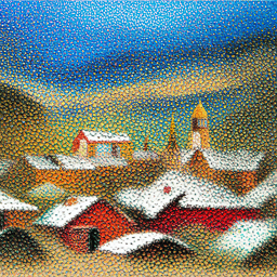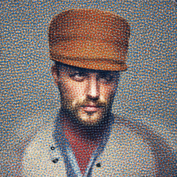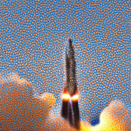an oil painting of a snowy mountain village (stage 2)	a man wearing a hat (stage 2)	a rocket ship (stage 2)

Step=15:

an oil painting of a snowy mountain village (stage 1)	a man wearing a hat (stage 1)	a rocket ship (stage 1)
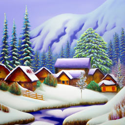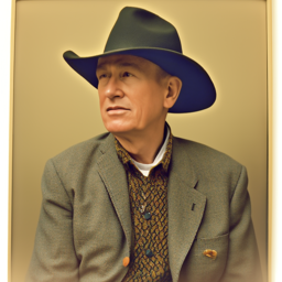an oil painting of a snowy mountain village (stage 2)	a man wearing a hat (stage 2)	a rocket ship (stage 2)

We can see that the images generated with more inference steps have significantly higher quality.

1.1 Implementing the Forward Process

To efficiently create a noised image in different time steps, I followed the formula below to do the forward process.

, where $ϵ\sim N(0,1)$$\epsilon \sim N(0,1)$, $x_0$ is the clean image and $x_t$$x_t$ is the noised image in the $t$$t$ time step.

Below are examples of different noise levels.

clean	$t=250$$t=250$	$t=500$$t=500$	$t=750$$t=750$

1.2 Classical Denoising

The classical denoising approach which uses Gaussian blur filtering can hardly give good results. Below are examples.

$t=250$$t=250$	$t=500$$t=500$	$t=750$$t=750$

1.3 One-Step Denoising

The pre-trained U-net which is trained to estimate the noise added in an image can denoise much better. Given the noised image at the time step $t$$t$ is $x_t$$x_t$ with an unknown noise $ϵ$$\epsilon$ , the estimated clean image ${\hat{x}}_0$$\hat x_0$ can be derived from the estimated noise $\widehat{ϵ}$$\hat \epsilon$ :

, where $\widehat{ϵ}$$\hat \epsilon$ is the noise estimated by the U-net. The ${\hat{x}}_0$$\hat x_0$ is our one-step denoising result. Below are examples.

	Clean	$t=250$$t=250$	$t=500$$t=500$	$t=750$$t=750$
Image in various noise level
One-step denoise result	N/A

1.4 Iterative Denoising

We can also use iterative denoising to get better results. I followed the provided formula to compute the estimated image in the previous time step.

, where $t^{\prime }=t-1$$t^\prime = t-1$ , ${\alpha }_t=\frac{{\overline{\alpha }}_t}{{\overline{\alpha }}_{t^{\prime }}}$$\alpha_t = \frac{\bar\alpha_t}{\bar\alpha_{t'}}$ , ${\beta }_t=1-{\alpha }_t$$\beta_t = 1 - \alpha_t$ , and ${\hat{x}}_0$$\hat x_0$ is our current estimate of the clean image. The image gradually became less noisy during the denoising loop.

Compared with other approaches:

Original	Noised	Iterative denoised	One-step denoised	Gaussian filter

1.5 Diffusion Model Sampling

Using pure noises, I sampled random images from the diffusion model with the prompt "a high quality photo."

1.6 Classifier Free Guidance

The Classifier-Free Guidance is to estimate two noises in every iteration. One of them ${ϵ}_u$$\epsilon_u$ is unconditional (denoised without prompt) and the other one ${ϵ}_c$$\epsilon_c$ is conditional (denoised with prompt). Then, we can derive the guided noise $ϵ$$\epsilon$:

, where $\gamma =7$$\gamma = 7$ in our setting.

I used "a high quality photo" as a conditional prompt and "" as an unconditional prompt. Below are the results.

This gives us much better images compared to the images from the last section.

1.7 Image-to-image Translation

I leveraged the CFG to edit the existing images. I first noised the original image in different levels, and iteratively denoised them with CFG. Below are examples.

Noise level	1	3	5	7	10	20	Original
Campanile
Professor
UC Berkeley

1.7.1 Editing Hand-Drawn and Web Images

I used this procedure on non-realistic images (web images and hand-drawn images).

Noise level	1	3	5	7	10	20	Original
Frieren

1.7.2 Inpainting

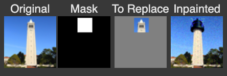
By using mask, we can keeps some area in the images unchanged during the denoising process. Formally, the image $x_t$$x_t$ at time step $t$$t$ is obtained by:

, where $\mathbf{m}$$\bold m$ is a binary mask with values of $[0,1]$$[0, 1]$.

1.7.3 Text-Conditional Image-to-image Translation

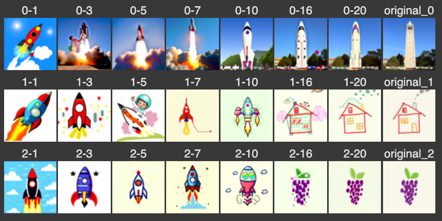
I used "a rocket ship" as a conditional prompt to translate my images into rocket ships. The process was done by using iterative CFG mentioned in section 1.6. The only thing different was the conditional prompt.

1.8 Visual Anagrams

To generate images look like one thing in a side and look like another thing when flipped upside down, we can denoise with the average of two noises. One of them is the "normal noise" and the other one is the "flipped noise".

, where $p_1,p_2$$p_1, p_2$ are the prompts.

an oil painting of people around a campfire	an oil painting of an old man
a pencil	a rocket ship
a lithograph of waterfalls	a lithograph of a skull

1.9 Hybrid Images

Similarly, processing on two estimated noises and averaging them allows us to play different tricks. Therefore, performing low-pass and high-pass filtering on the noises can give us hybrid images.

skull(far) + waterfall(close)	a man wearing a hat + a rocket ship	a photo of a man + a photo of the amalfi coast

For the low-pass filtering, I used kernel size = 33 and sigma = 2.

Part B

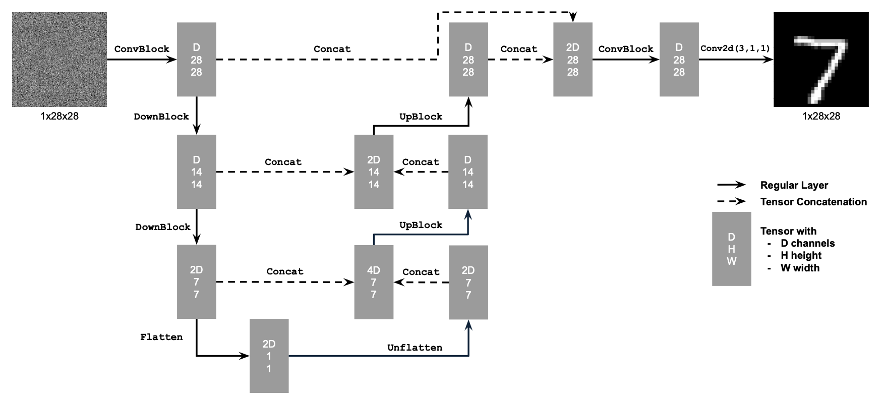
1.1 Implementing the UNet

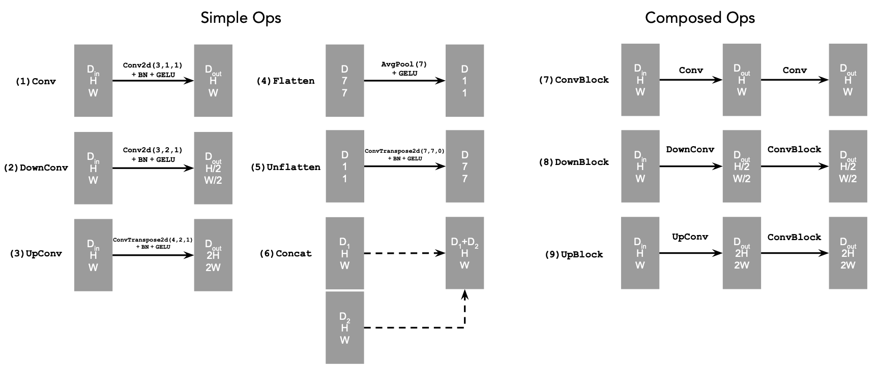
I followed the figures and instructions on the project description to implement the UNet. The architecture of the UNet is defined as follow:

1.2 Using the UNet to Train a Denoiser

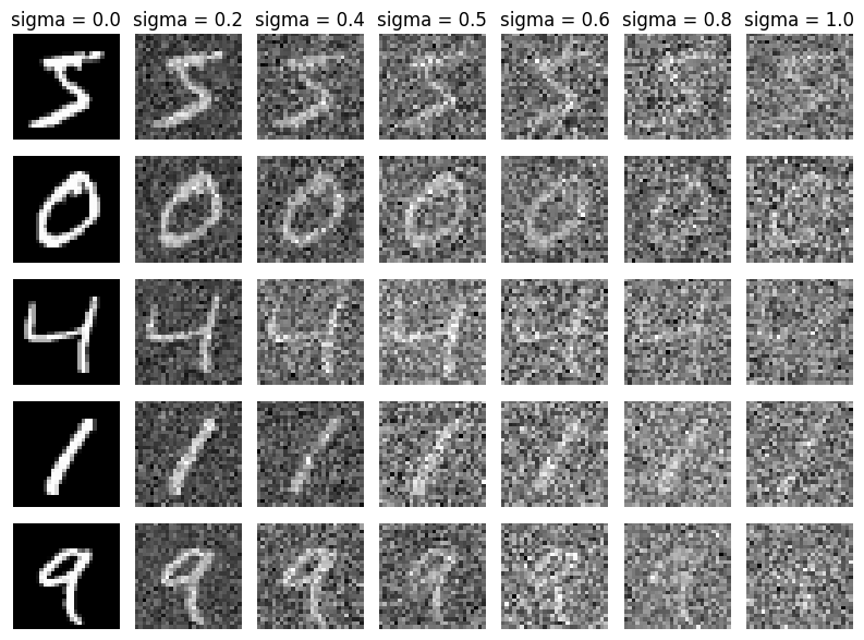
To train an UNet as a denoiser, I used the gaussian noise to add noise to images. Below are some examples that add Gaussian noise to MNIST dataset.

1.2.1 Training

I trained an one-step denoiser to denoise noisy images. The noisy images were obtained by adding gaussian noise with $\sigma =0.5$$\sigma=0.5$ to clean images.

Hyper-parameters:

xxxxxxxxxx
4
1
Epoch: 5
2
Batch size: 256
3
Optimizer: Adam
4
Learning Rate: 1e-4
4
Learning Rate: 1e-4

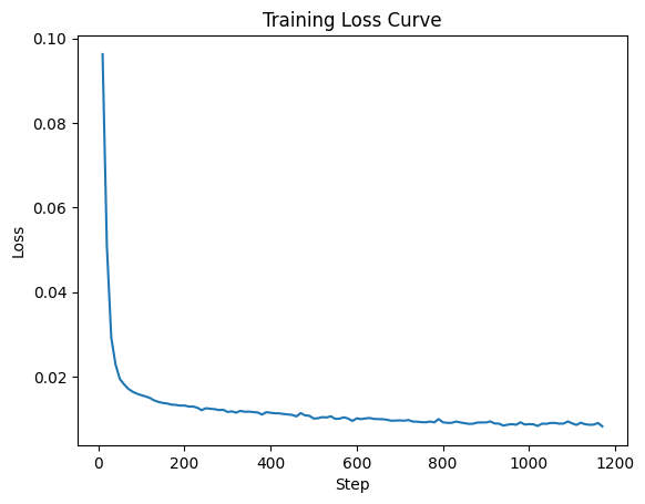
I logged the loss every 10 steps to plot the loss curve.

Loss curve
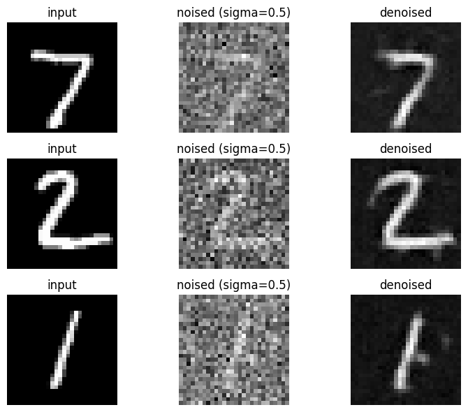Results after training 1 epoch
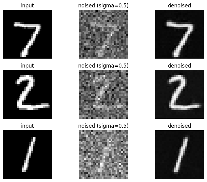Results after training 5 epochs

1.2.2 Out-of-Distribution Testing

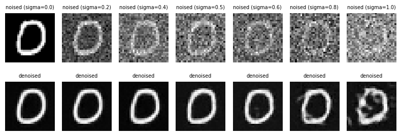
Since my denoiser is trained on MNIST digits noised with $\sigma =0.5$$\sigma=0.5$ . It shouldn't perform as good when denoising the digits noised with different $\sigma$$\sigma$ .

2.1 Adding Time Conditioning to UNet

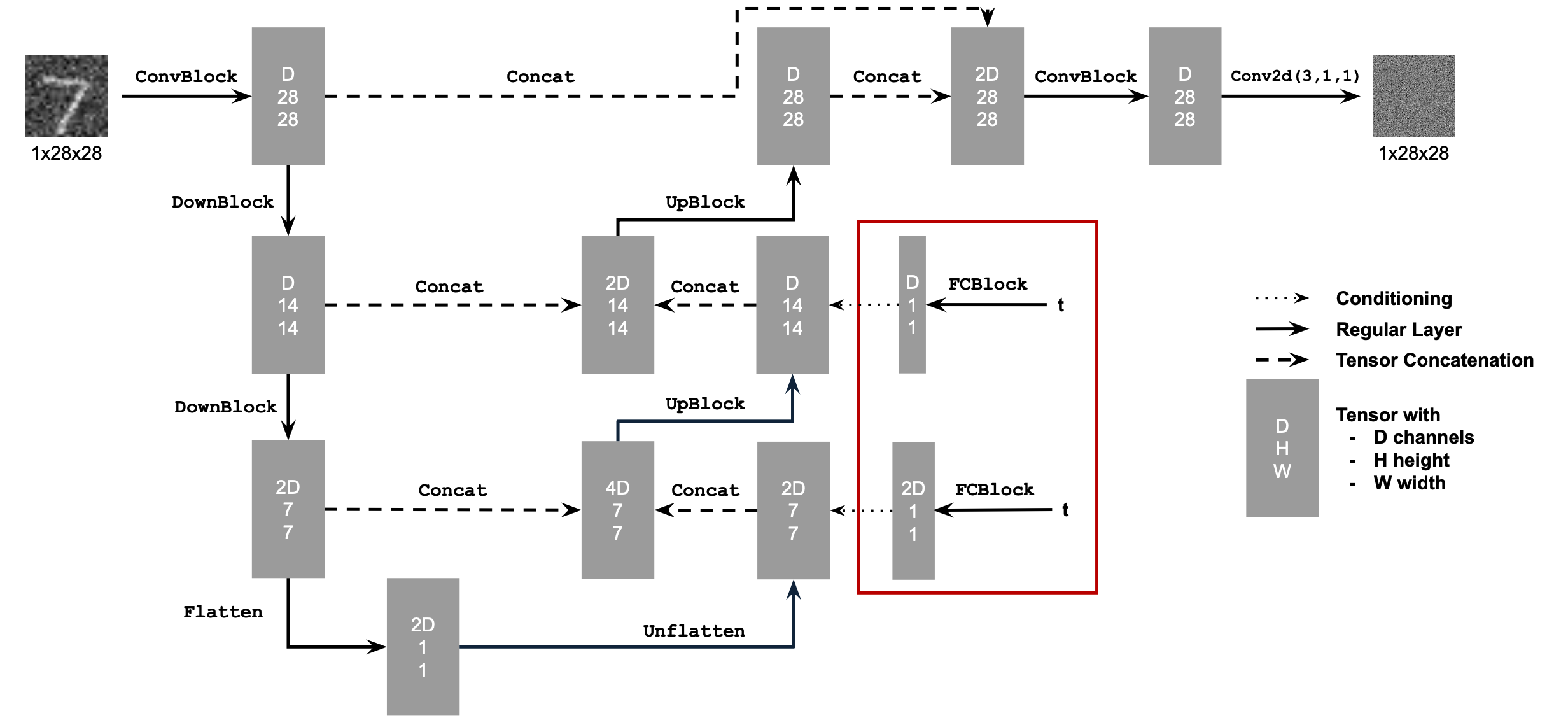
To train a diffusion model that estimate the noise at every time step, I started with adding time conditioning to UNet (as project description suggested). This is done by adding two fully-connected layers to the UNet.

2.2 Training the UNet

I used the hyper-parameters below:

xxxxxxxxxx
4
1
Epoch: 20
2
Batch size: 128
3
Optimizer: Adam with exponential decay scheduling (gamma = 0.1^(1/20))
4
Learning Rate: Start at 1e-3
2
Batch size: 128

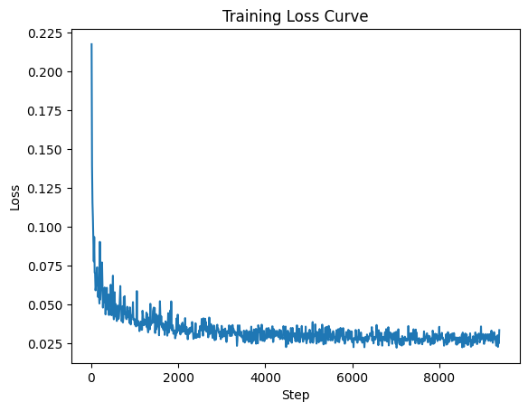
I logged the loss every 10 steps to plot the loss curve.

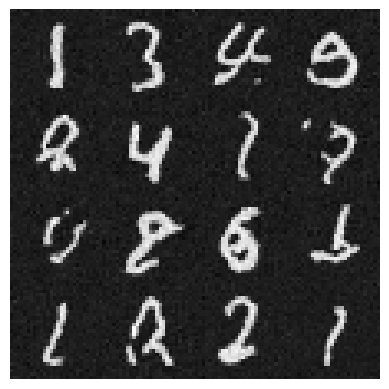
2.3 Sampling from the UNet

The time-conditional sampling is similar to section 1.4 in Part A.

I used this equation to iteratively denoise. Below are examples.

Results after training 5 epochs
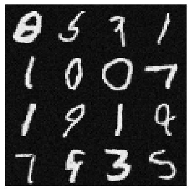Results after training 20 epochs

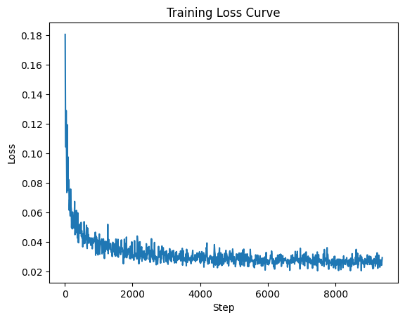
2.4 Adding Class-Conditioning to UNet

Class-conditioning is added to UNet by adding two fully-connected layers. During the training process, I passed class labels into the model. That is, $\widehat{ϵ}=\text{UNet}(x_t,t,c)$$\hat\epsilon = \text{UNet}(x_t, t, c)$, where $t$$t$ is the time step and $c$$c$ is the class label. Also, the class labels were set to $\mathbf{0}$$\bold 0$ with $10\mathrm{\%}$$10\%$ probability to make the UNet to work in unconditional cases.

Training hyper-parameters:

xxxxxxxxxx
4
1
Epoch: 20
2
Batch size: 128
3
Optimizer: Adam with exponential decay scheduling (gamma = 0.1^(1/20))
4
Learning rate: start at 1e-3
1
Epoch: 20

I logged the loss every 10 steps to plot the loss curve.

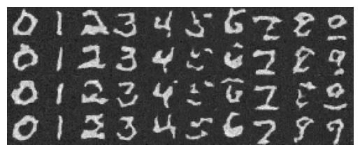
2.5 Sampling from the Class-Conditioned UNet

The sampling was very similar to section1.6 in Part A. Using CFG to guide the model do the class-conditioned estimates.

Results after training 1 epoch
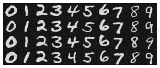Results after training 5 epochs
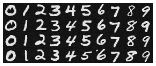Results after training 20 epochs