Project 4A

Shoot and Digitize Pictures

The pictures to merge are:

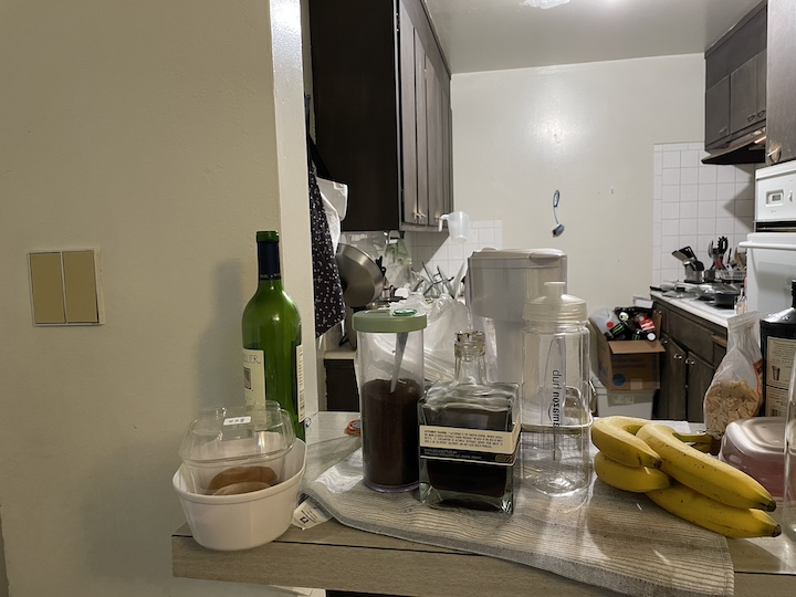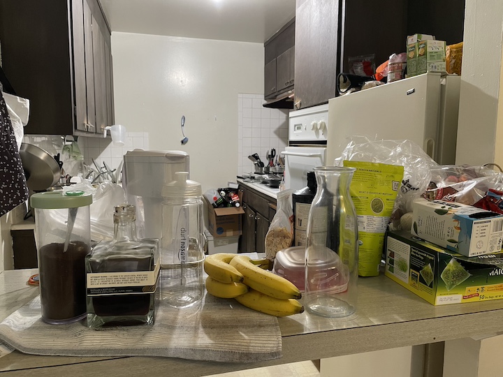Kitchen (left)	Kitchen (right)
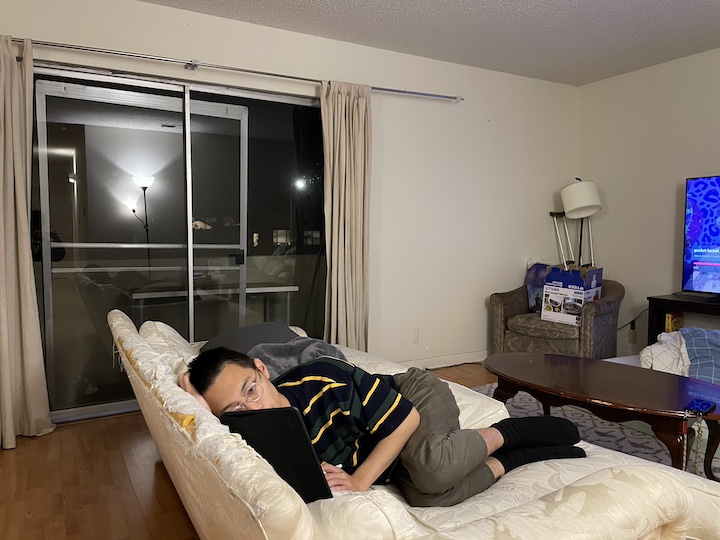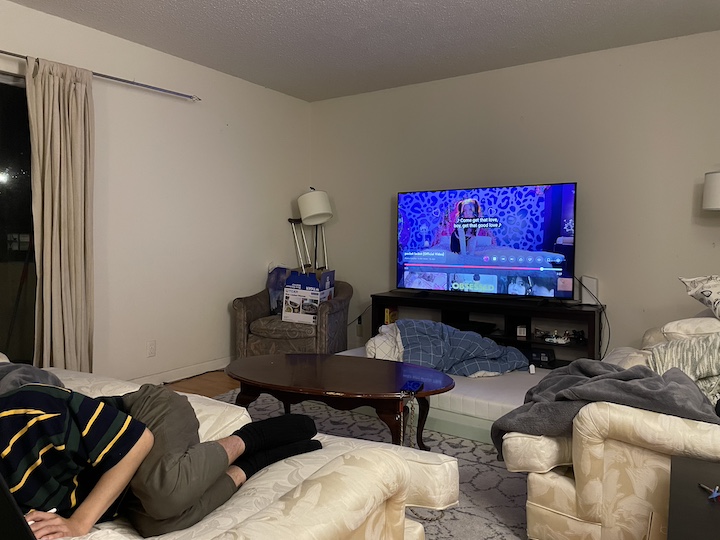Living room (left)	Living room (right)
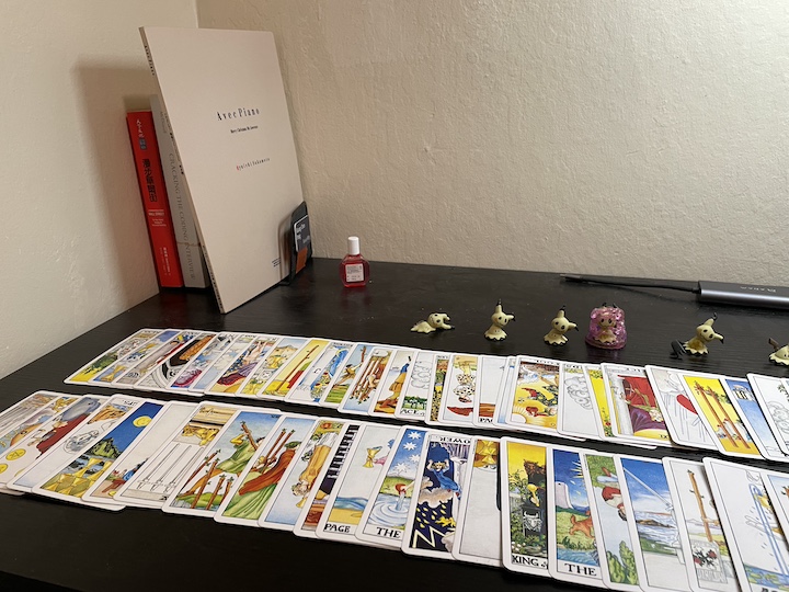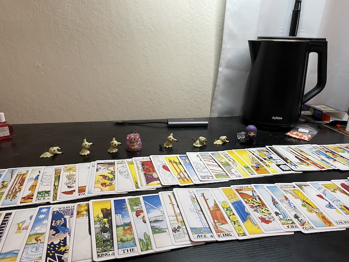Desk with tarot cards (left)	Desk with tarot cards (right)

Pictures to rectify are:

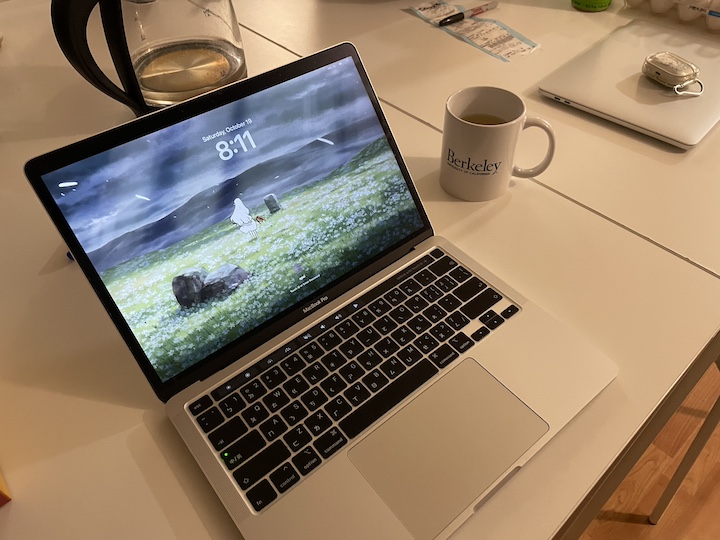Laptop (16:9)
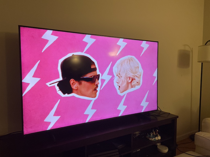Television (16:10)

Recover Homographies

In this part, we want to find the matrix $H$$H$ such that

, where $x,y$$x, y$ is the point coordinate in the source image, and $x^{\prime },y^{\prime }$$x', y'$ is the point coordinate in the target image.

Expanding the equation, we have:

then solve the formula:

Now we can use the least square errors to estimate the matrix $H$$H$ by applying at least 4 corresponding points to the equation.

Warp the Images

After computing the matrix $H$$H$, I used inverse warping with bilinear interpolation to warp project the image to the target project plane.

The coordinates after inverse warping should be translated to fit in a new canvas. Therefore, I find the minimal $x,y$$x, y$ values and translate the whole image with that $x,y$$x, y$ values and the new canvas size is then determined by ($x_{max},y_{max}$$x_{max}, y_{max}$).

We are able to rectify the images now:

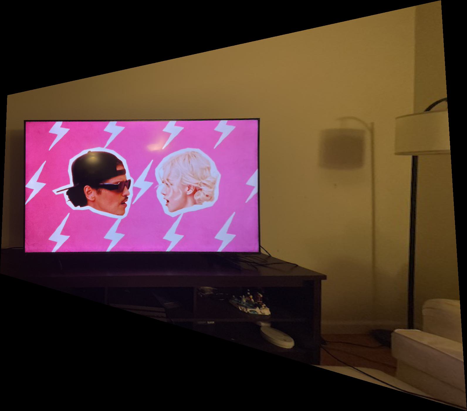Television	Rectified television
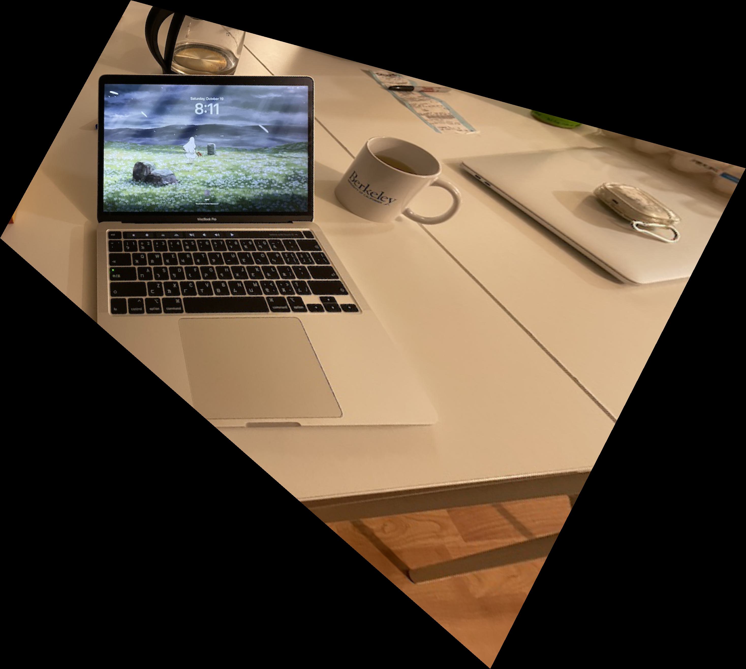Laptop	Rectified Laptop

Blend images into a mosaic

Finally, we can build a panorama by warping corresponding points to the same coordinates.

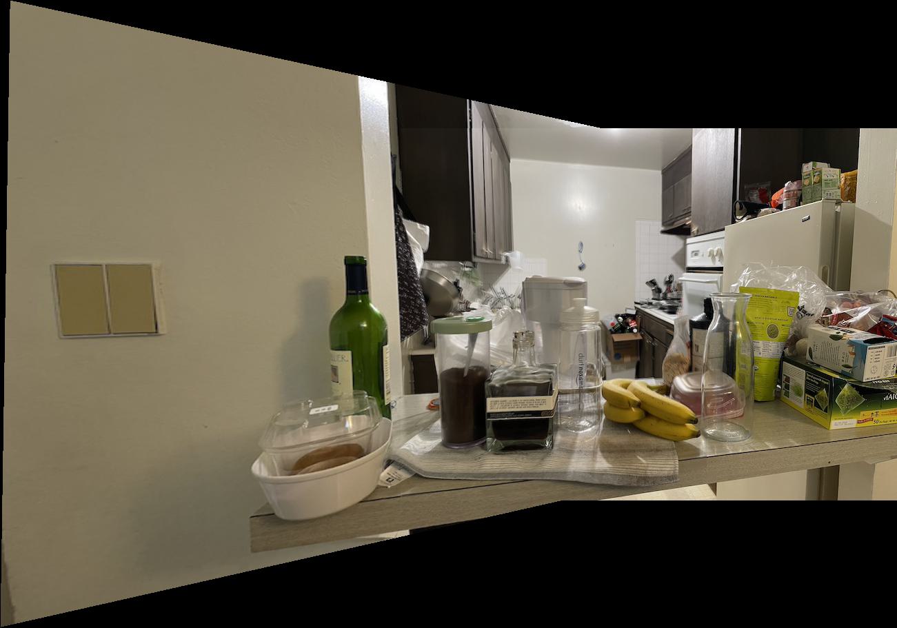
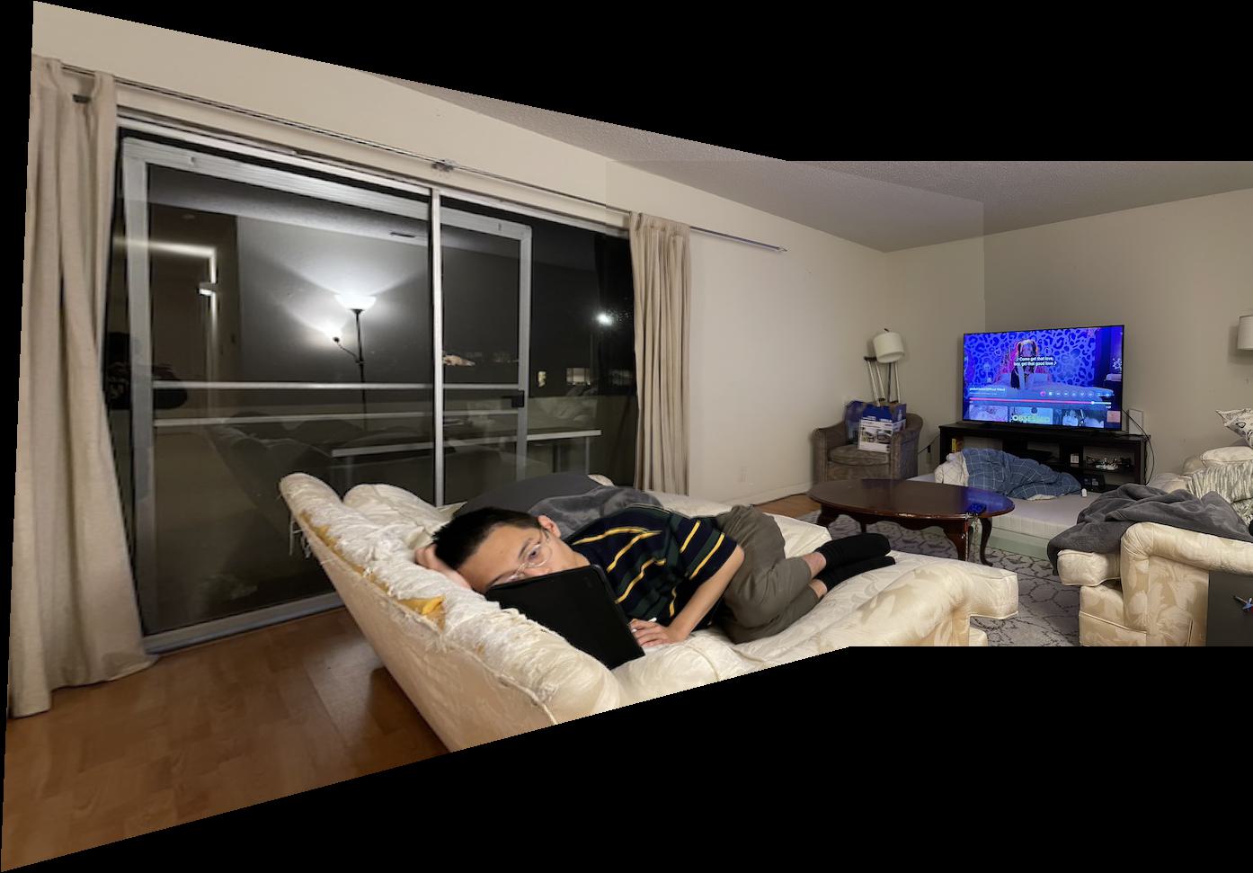
I first tried naive averaging in the intersecting part of two images:

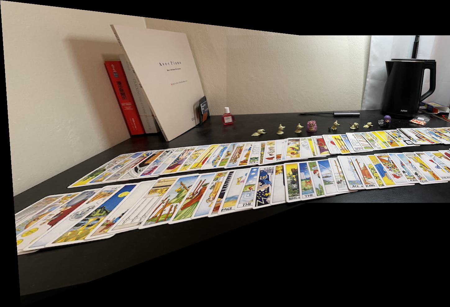The naive averaging didn't give preferable results, specifically, there are clear lines resulting from naive averaging in the blended image.

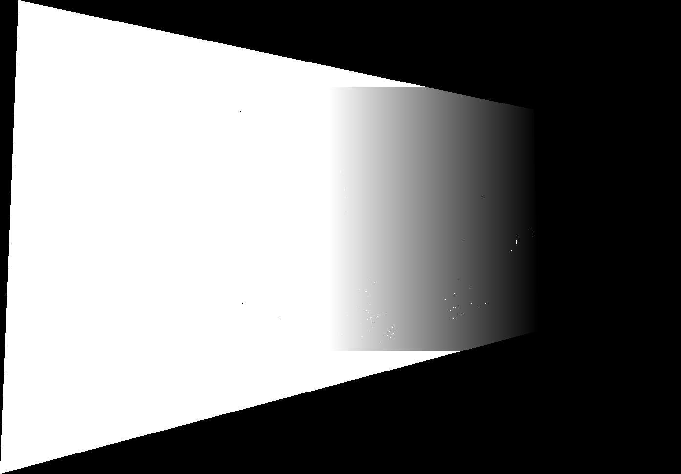
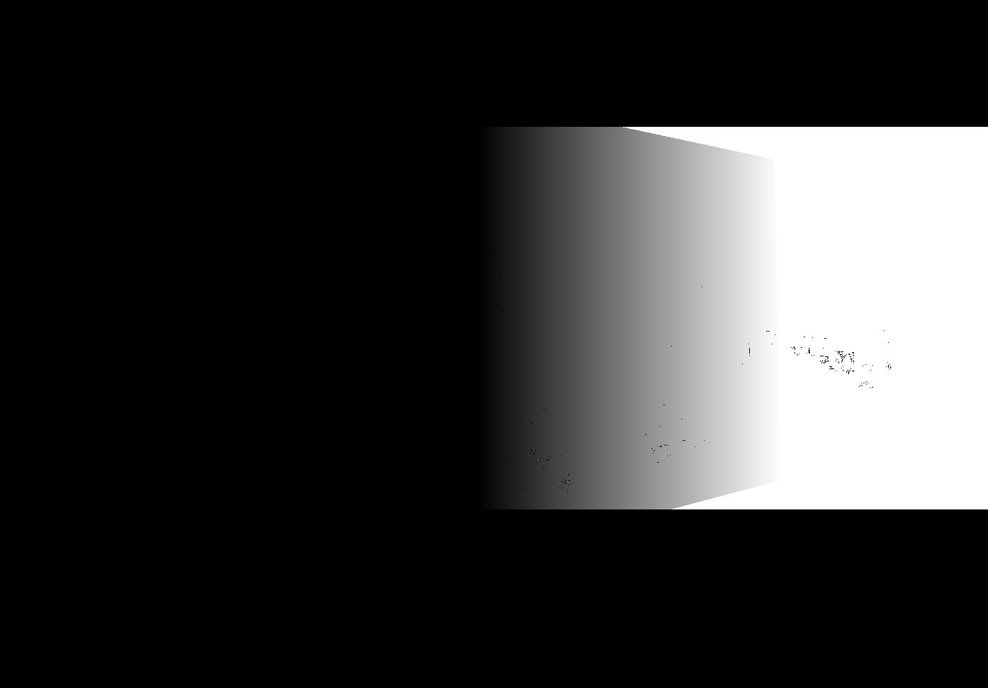
Therefore, I used the weighted averaging as my second approach. The weights of intersecting parts are determined by a linear function, where the leftmost part has a weight of 0 and the rightmost part has a weight of 1. The weighting masks of the second image are shown below:

Left mask	Right mask

The subtle noises on the right mask resulted from the way I implemented it. I construct the mask by mask = np.any(image, axis=2). Thus, the black pixels in the image would generate the black pixels on the mask. However, it has no negative effect on our blending since the pixels are black and no blending is needed in those black pixels.

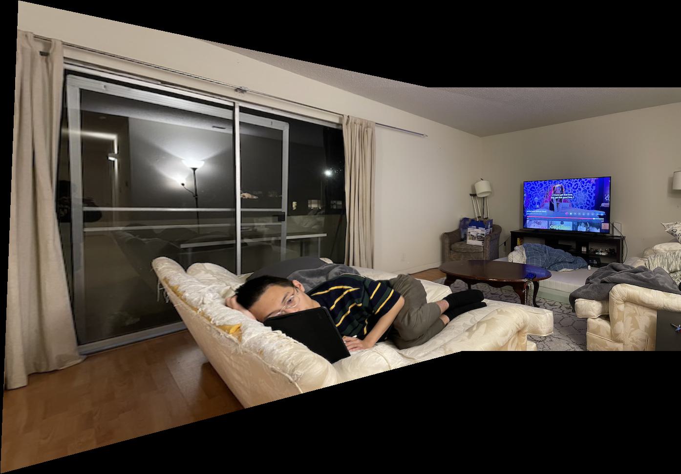
The results are:

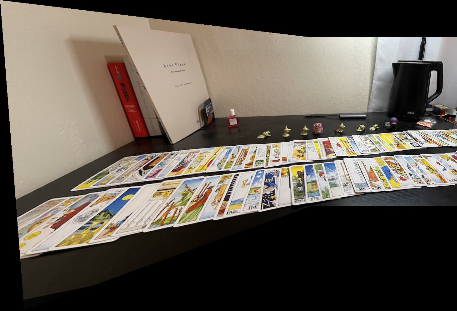The quality of the panoramas is much better than the naive averaged one.

Project 4B

In part B, the objective is to create a automatic stitching algorithm. It consists of several steps:

1. Detect corner features using Harris corner detector

2. Reduce feature points with Adaptive Non-Maximal Suppression (ANMS)

3. Extract feature descriptors from each feature point

4. Match feature descriptors

5. Use RANSAC to compute a homography

Harris Corners

I first applied Harris corner detector to find the feature points that look like corners. This resulted in many feature points in images.

Adaptive Non-Maximal Suppression

Since there is too many feature points from the previous step, I used Adaptive Non-Maximal Suppression (ANMS) to reduce the feature points but also keep the "useful" points that uniformly spread in the image.

I computed the pair-wise L2 distance for each feature points, and update the supression radius by the formula given by paper:

Then, I set the minimum supression radius with the 200th largest suppression radius to find 200 "useful" feature points from the images.

Generate Feature Descriptors

The feature descriptor of each feature point is a 64-dimensional vector. For each feature point, I used its surrounding, axis-aligned $40\times 40$$40\times 40$ pixels and downsampled them (with Gaussian blur) into $8\times 8$$8\times 8$. Then, normalized it so that the mean is $0$$0$ and the standard deviation is $1$$1$. Finally, they are flattened to be a 64-dimensional vector as a feature descriptor.

It looks like:

Match Feature Descriptors

I computed pair-wise L2-distance of feature descriptors, and only retained the feature descriptor pairs $(i,j)$$(i, j)$ such that:

, where $d_{i,j}$$d_{i, j}$ is the L2 distance between $i$$i$_th feature descriptor of the first image and the $j$$j$_th feature descriptor of the second image, and ${\mathbf{D}}_{mean},{\mathbf{D}}_{std}$$\bold D_{mean}, \bold D_{std}$ are the mean value and the standard deviation of the L2-distance of all feature descriptor pairs. By doing this, I filtered out roughly $93\mathrm{\%}$$93\%$ of noisy pairs.

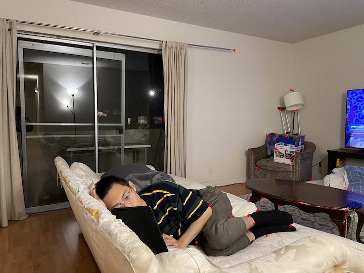
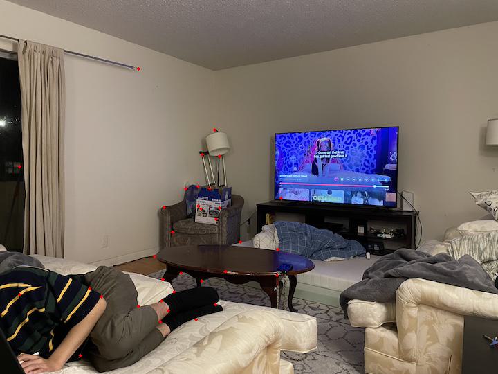
Furthermore, I used Lowe's 1-NN/2-NN algorithm to filter out noisy pairs. I chose the pairs with $\frac{e_{1-NN}}{e_{2-NN}}<0.25$$\frac{e_{1-NN}}{e_{2-NN}} < 0.25$ . The result is shown below:

RANSAC

Finally, I implemented RANSAC to give a robust homography. As described in the lecture, I randomly sampled 4 pairs, computed the homography, counted the inliers, and used the largest inlier set to compute the final homography.

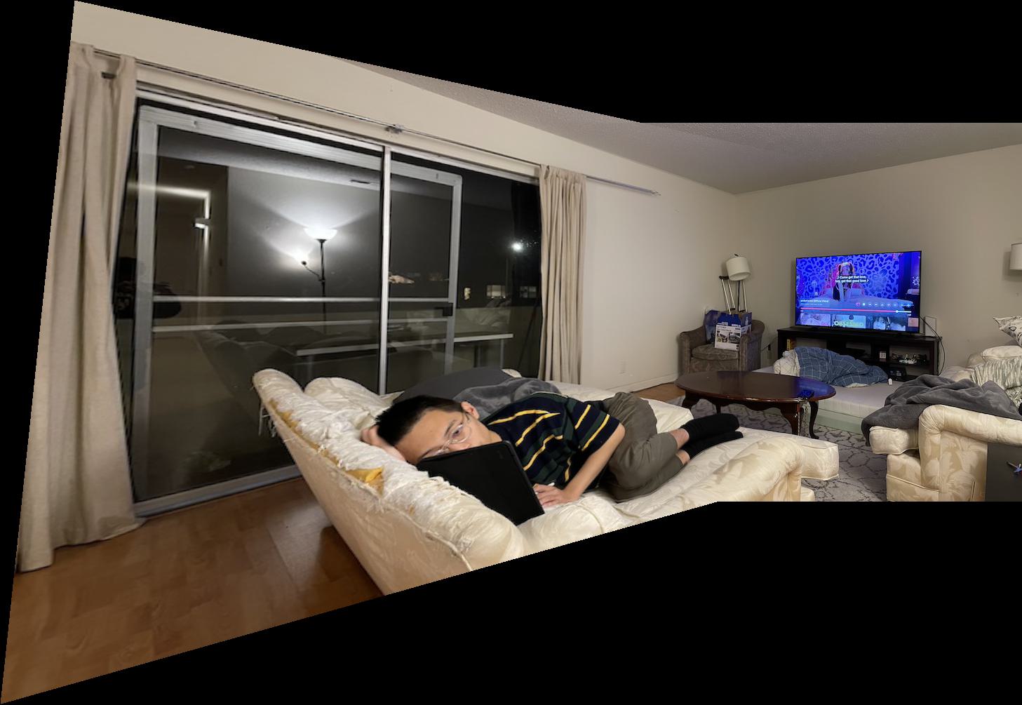
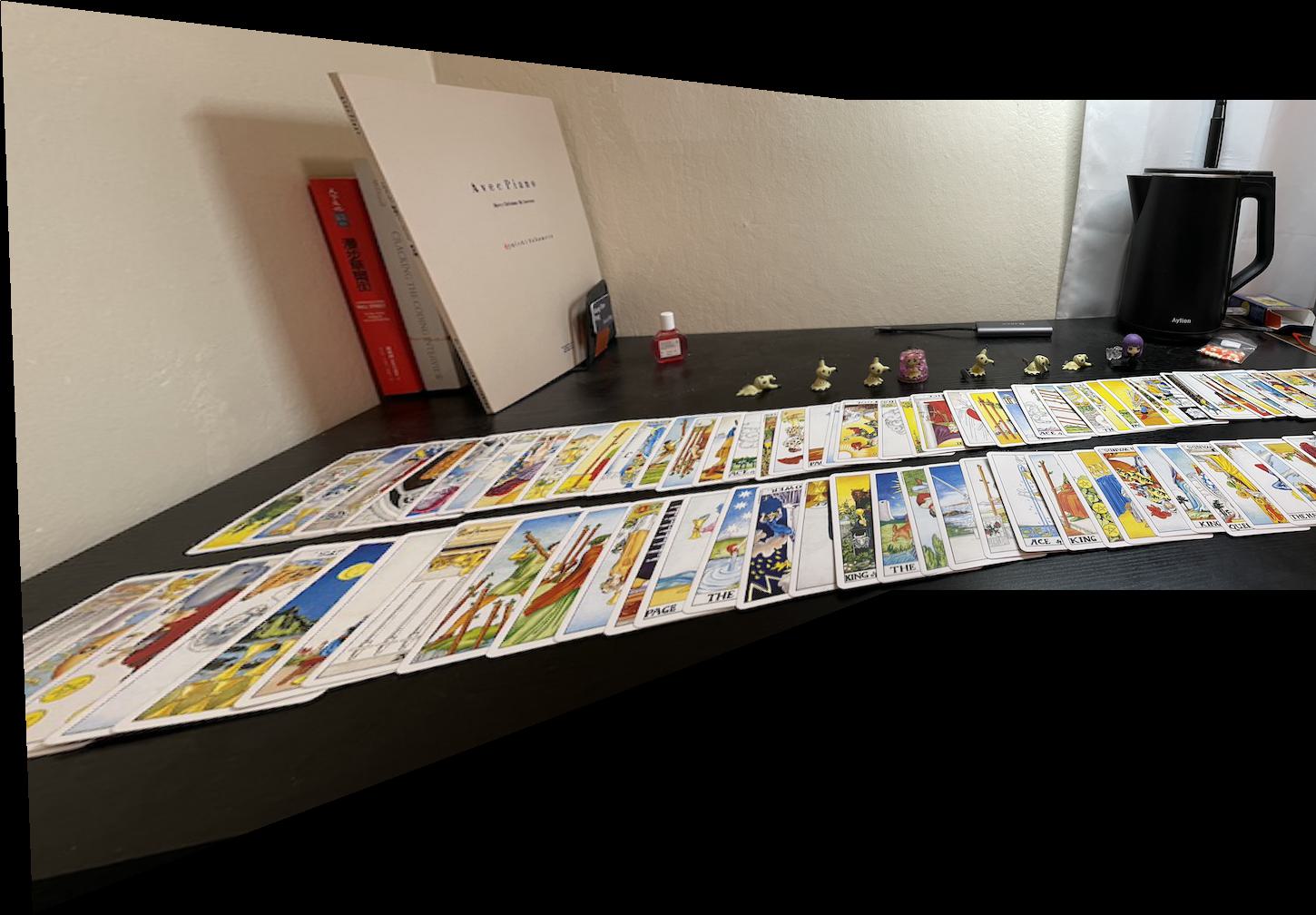
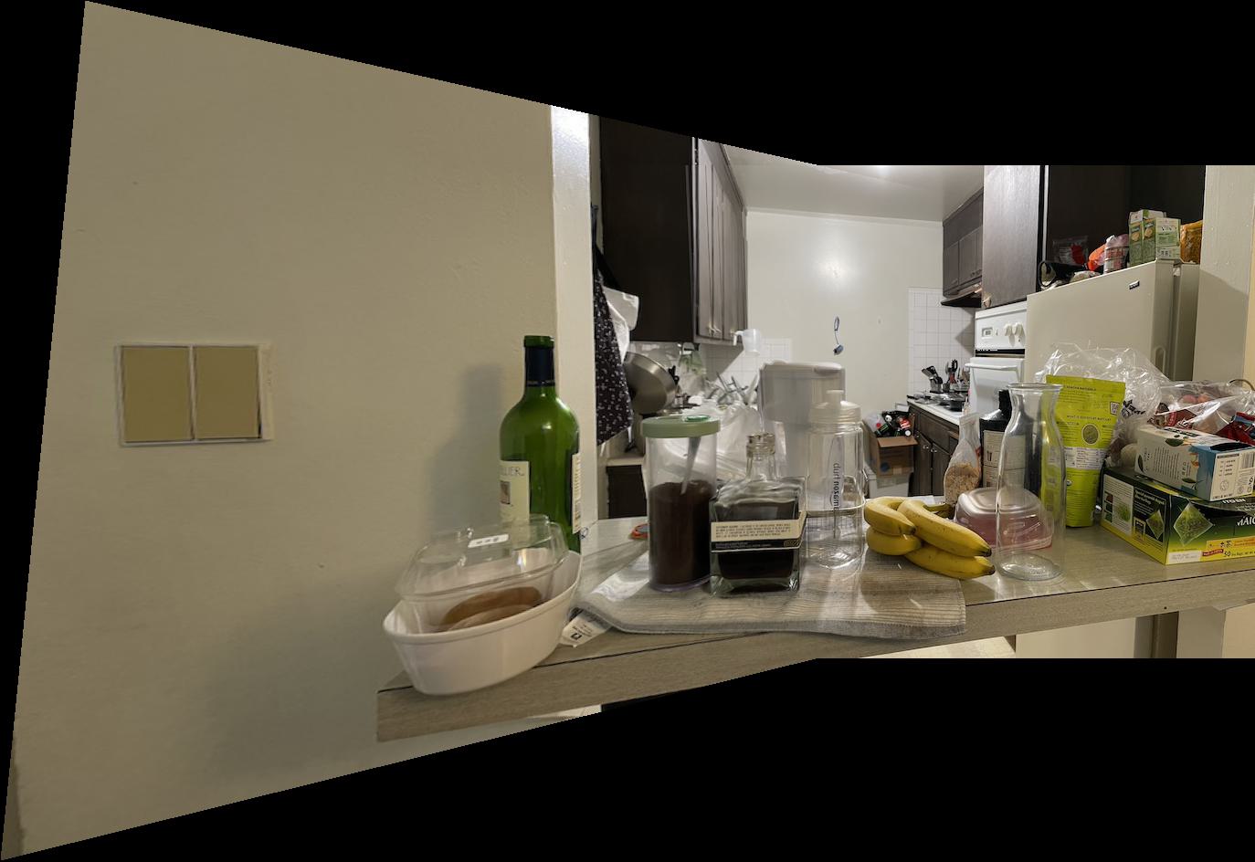
After doing RANSAC, we're able to mosaic the images now.

Belows are the final results:

Auto	Manual
Auto	Manual
Auto	Manual

What have you learned?

I found that it is very interesting to use a random algorithm (RANSAC) to generate robust results. The power of randomness is amazing.