CS 280A HW2 Report
CS 280A HW2 Report1.1: Finite Difference Operator1.2: Derivative of Gaussian Filter2.1: Image "Sharpening"2.2: Hybrid Images2.3: Gaussian and Laplacian Stacks2.4: Multiresolution Blending
1.1: Finite Difference Operator
To obtain the difference between adjacent pixels of an image
 |  |
|---|---|
Note that the range of the convoluted image's pixels are
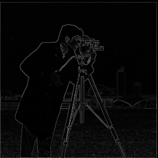
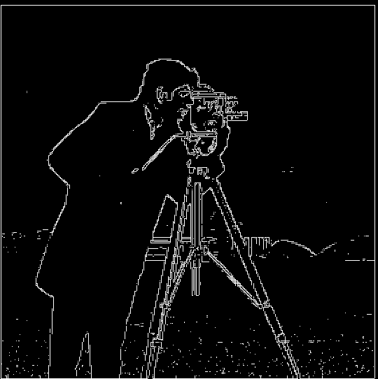
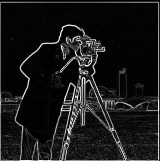
Next, the gradient magnitude image
 |  |
|---|---|
1.2: Derivative of Gaussian Filter
To remove noises generated by the lawn in the image, I convoluted the original image
 |  |
|---|---|
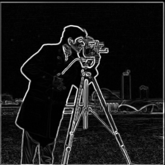 | 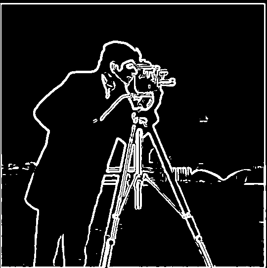 |
By applying Gaussian blur to the image, I saw the difference that the noises generated by the lawn are suppressed. This is mainly because the areas of the gradients generated by lawn are small. Therefore, they can be smoothed by the Gaussian blur and not be considered an "edge."
Notice that
Now, compute
 |  |
|---|---|
 |  |
Now we verified that
2.1: Image "Sharpening"
Based on the fact that the Gaussian filter behaves like a low-pass filter, we can obtain the high frequencies
Since
, where
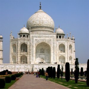
In the following examples, I chose
 | +3 | 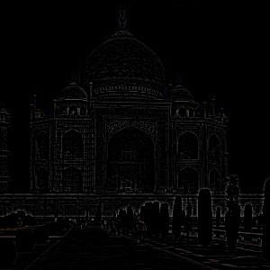 | = | 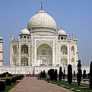 |
 | +3 |  | = |  |
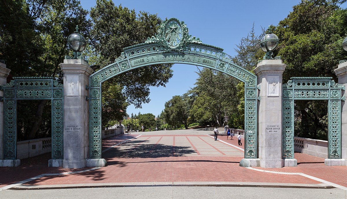
I picked an image of Sather Gate. I blurred it first and tried to resharpen it based on the blurred image.
 |
|---|
| Origin |
 |
| Blurred |
 |
| Resharpened |
Unfortunately, the resharpen process failed to "restore" the blurred image. The characters on the Sather Gate are still vague after resharpening.
2.2: Hybrid Images
To generate a hybrid image, given two images
, where
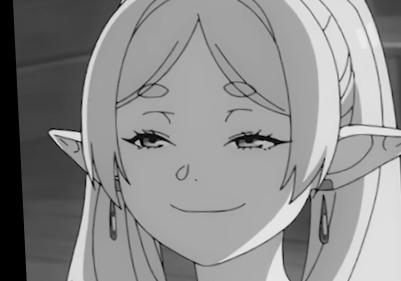
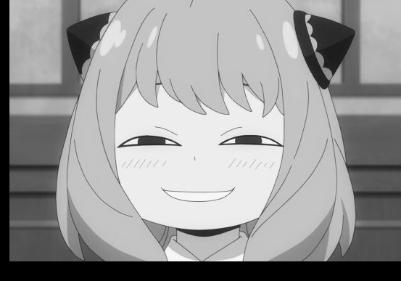
For example, take the following images as
 |  |
|---|---|
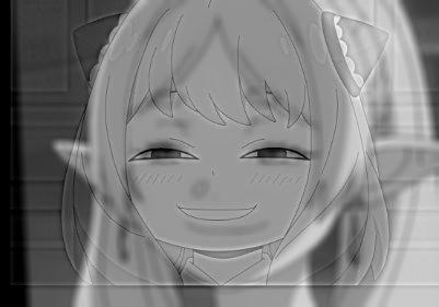
I kept the low frequencies of Frieren and the high frequencies of Anya to generate the hybrid image "Frierenya":
 |
|---|
| "Frierenya" |
The image looks more like Frieren when you look far away, while it looks more like Anya when you look close.
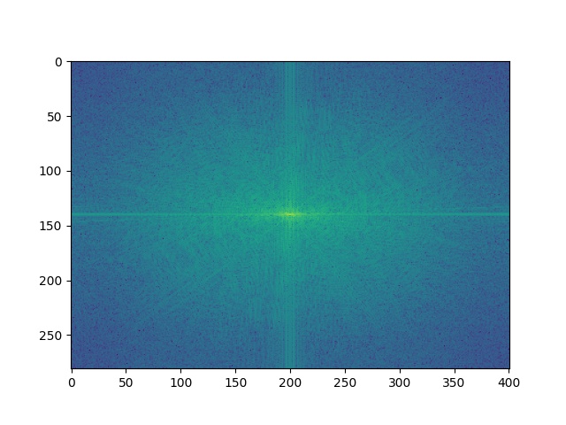
Now, let's inspect the frequencies of these images by Fourier analysis.
 | 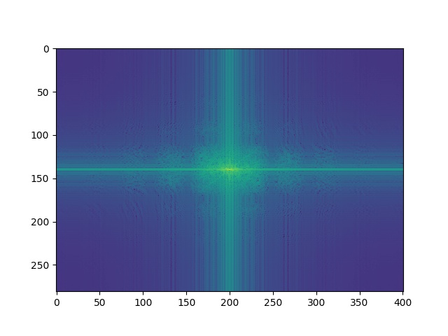 |
|---|---|
| Frieren's frequencies | Low frequencies of Frieren |
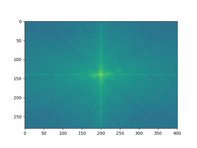 | 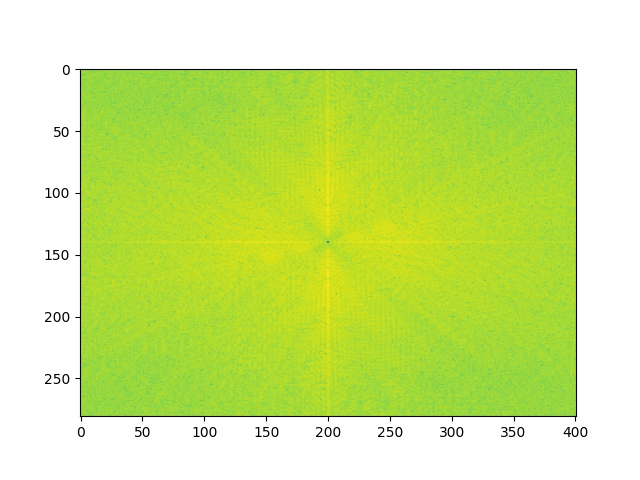 |
| Anya's frequencies | High frequencies of Anya |
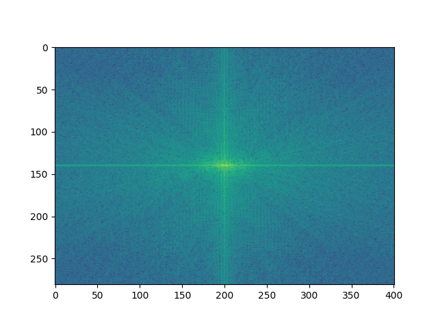 |
|---|
| Frierenya's frequencies |
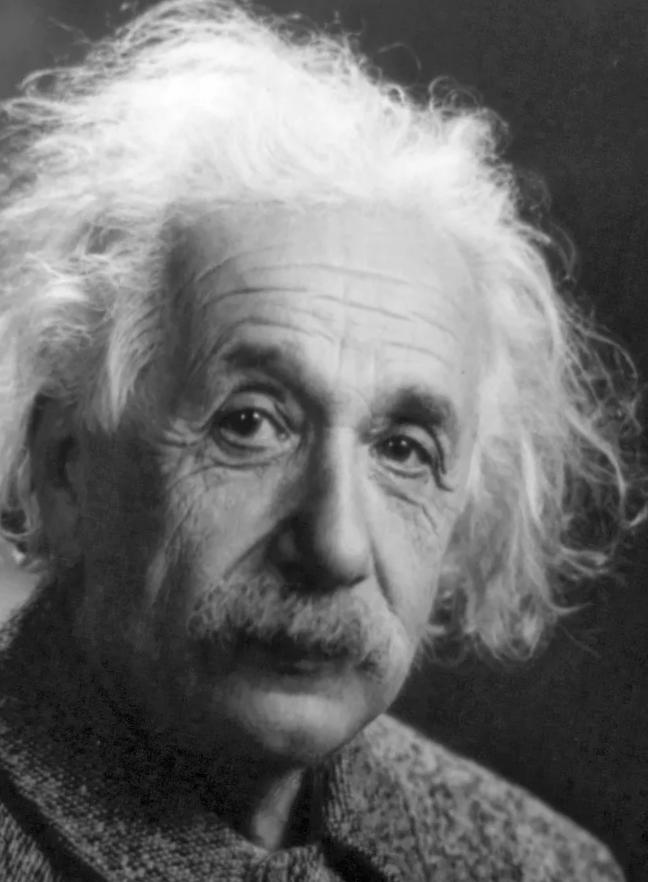
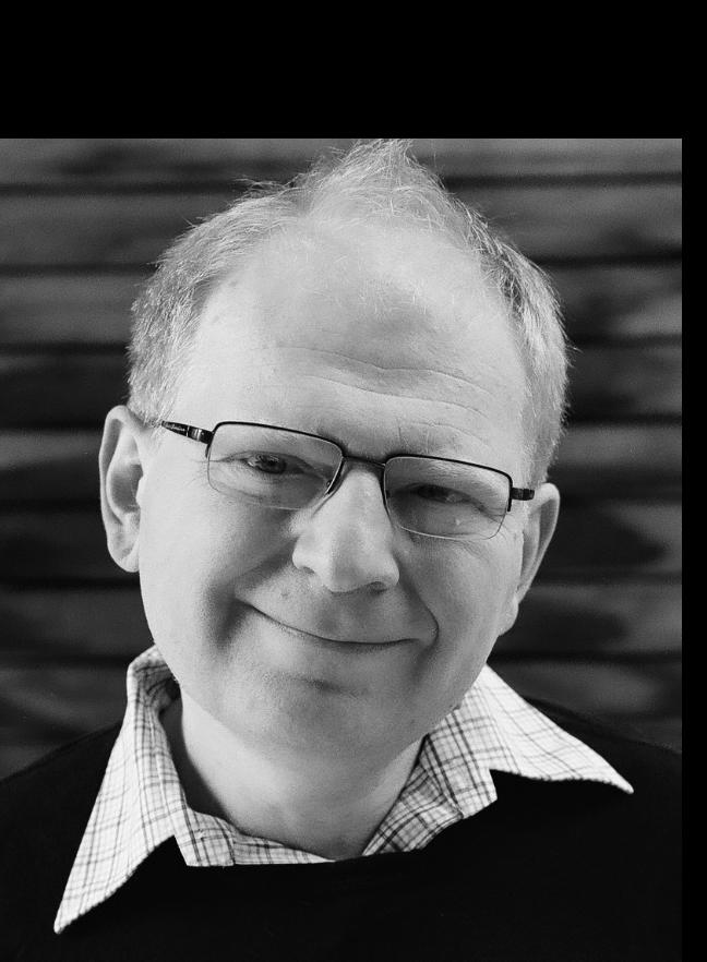
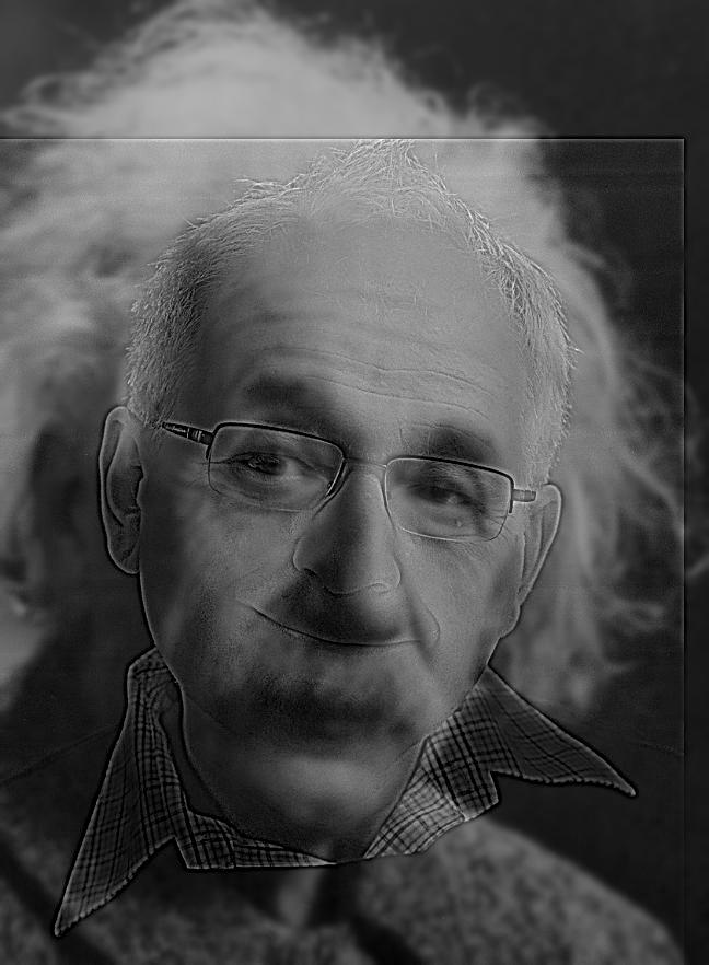
Similarly, I applied the merge process to two more pairs of images.
 |  |
|---|---|
 |
|---|
| "Albert Efros" |
The result seems acceptable, though Prof. Efros' collar aligned with Einstein's chin because of Einstein's large head (note that their eyes are aligned!).
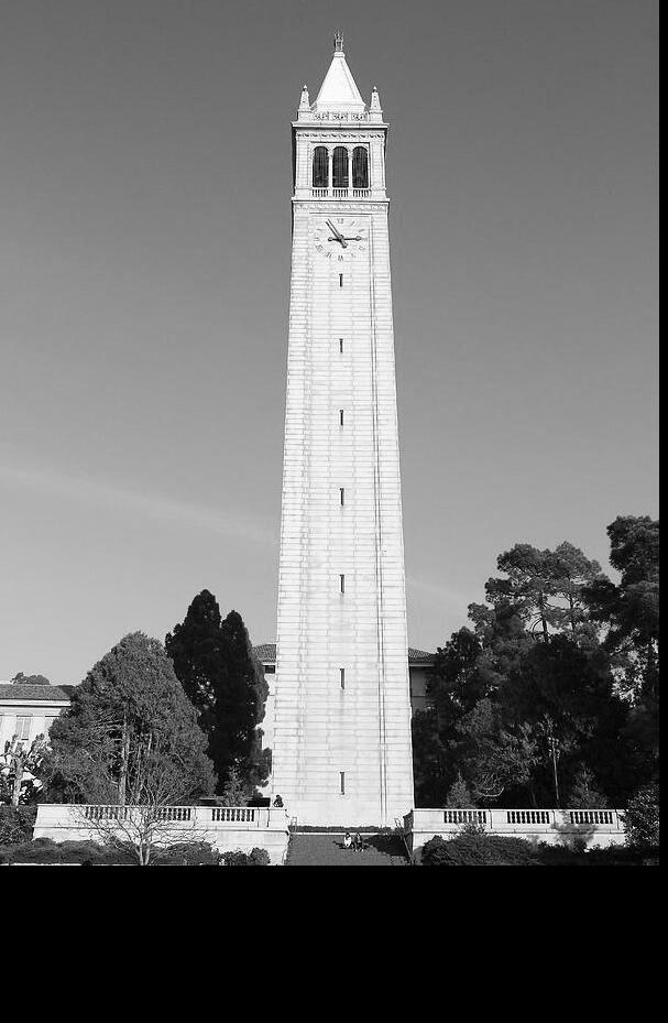
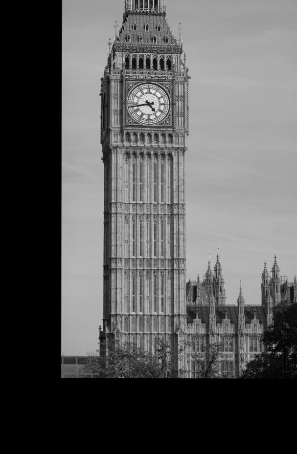
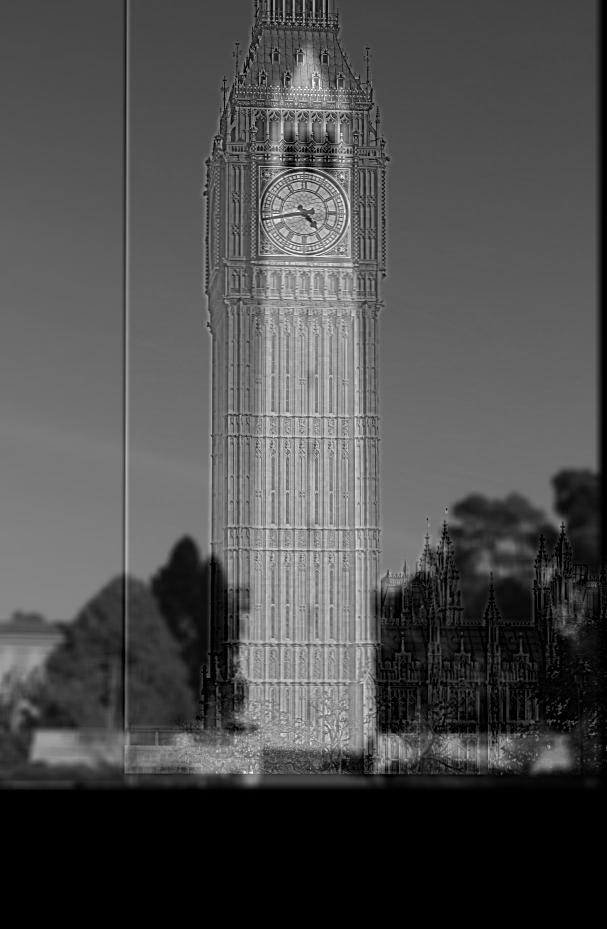
The following is a failed example:
 |  |
|---|---|
| Campanile | Big Ben |
 |
|---|
| "???????" |
For me, it seems like some strange texture on the surface of Campanile. I can't discern Big Ben through this image.
2.3: Gaussian and Laplacian Stacks
For the purpose of blending images, we need to compute their Gaussian stack and Laplacian stack first. Let the image be
, where
In my implementation, the kernel size of the Gaussian filter increased doubly as the level increased by one to capture the image's features in various scales.
The Laplacian stack can be derived from the Gaussian stack. It is defined as:
where
The original image can be constructed by summing up the Laplacian stack.
The following are the Laplacian stack examples of an apple and orange:
 |  |
|---|---|
For the first five levels of the Laplacian stack (Level 0 ~ Level 4), since the value of each pixel ranged from
 |  |
|---|---|
We also need a Gaussian stack of a mask to blend two images. In the "oraple" example, a mask that vertically divides the image is needed:

The Laplacian stack of the blended image can be computed by the formula:
, where
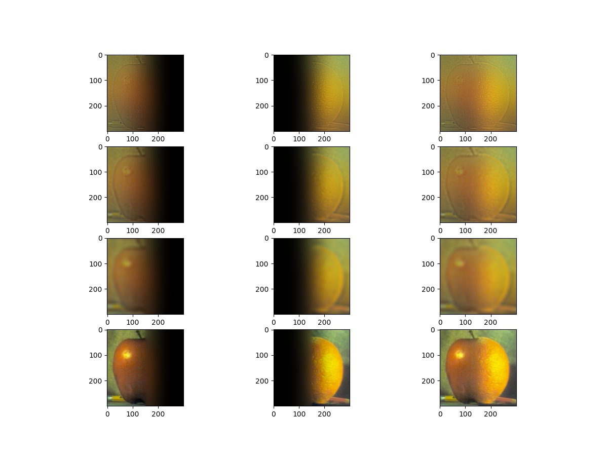
Finally,
 |
|---|
| Blending process |
The first three rows are levels 0, 2, and 4. The last row is the summation of the stack.
The columns are the different levels of
For better visualization, the images in the last level of the Laplacian stack are added to the images in the first three rows. For instance, the top-left image is
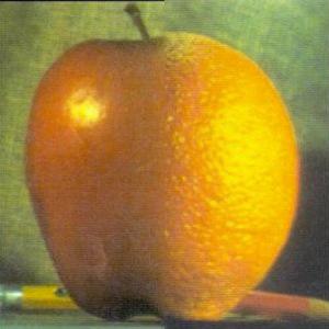
The final result is:
2.4: Multiresolution Blending
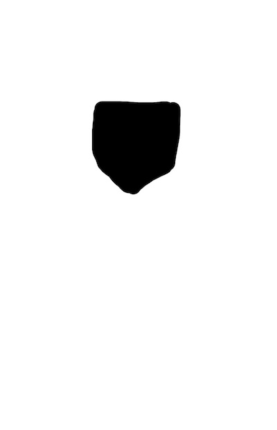
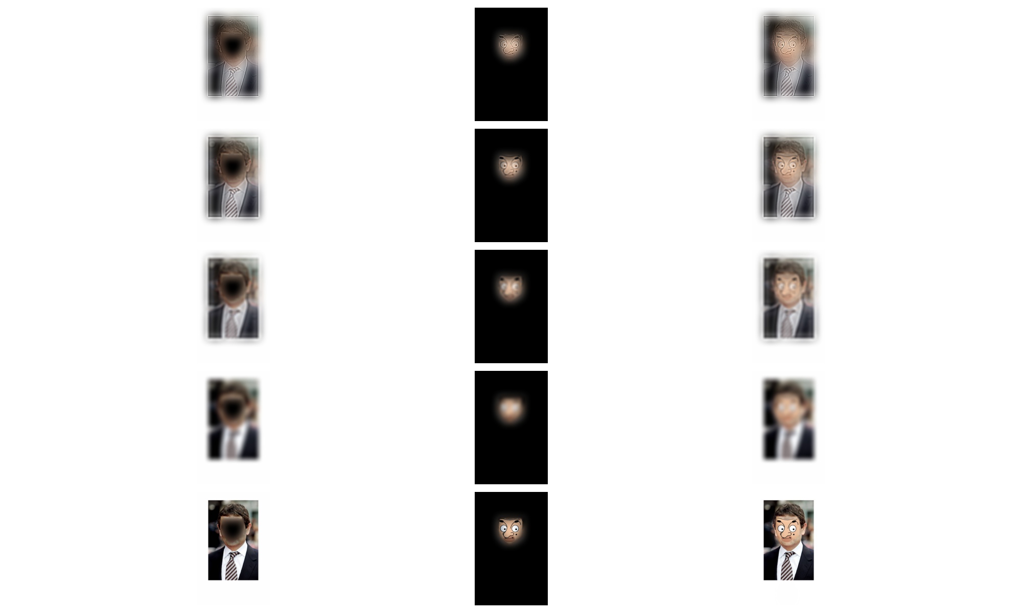
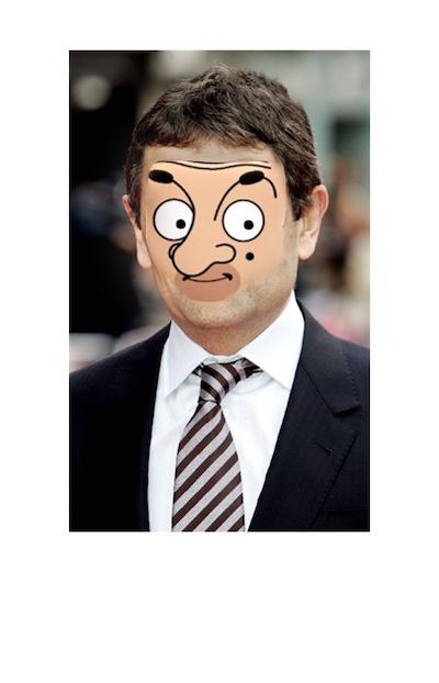
As described in section 2.3, we can blend arbitrary image pairs with an appropriate mask.
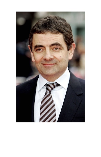
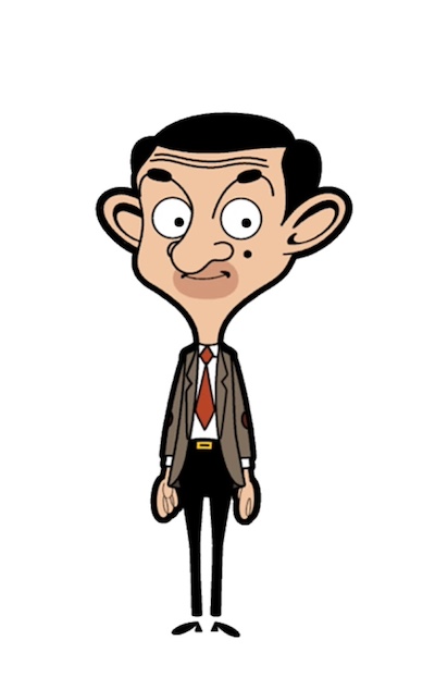
Mr. Bean
 |  |  |
|---|
 |
|---|
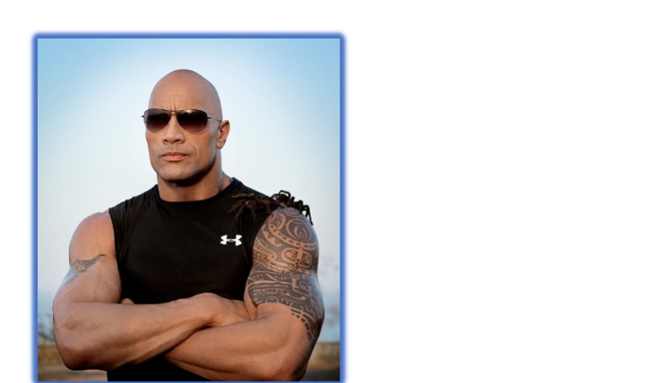
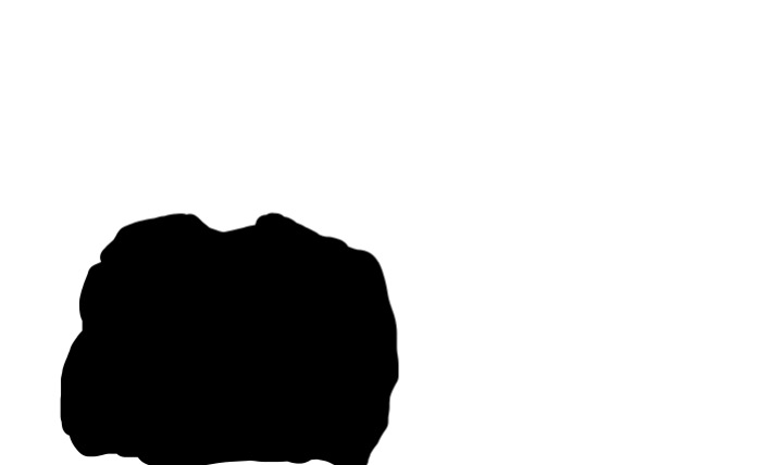
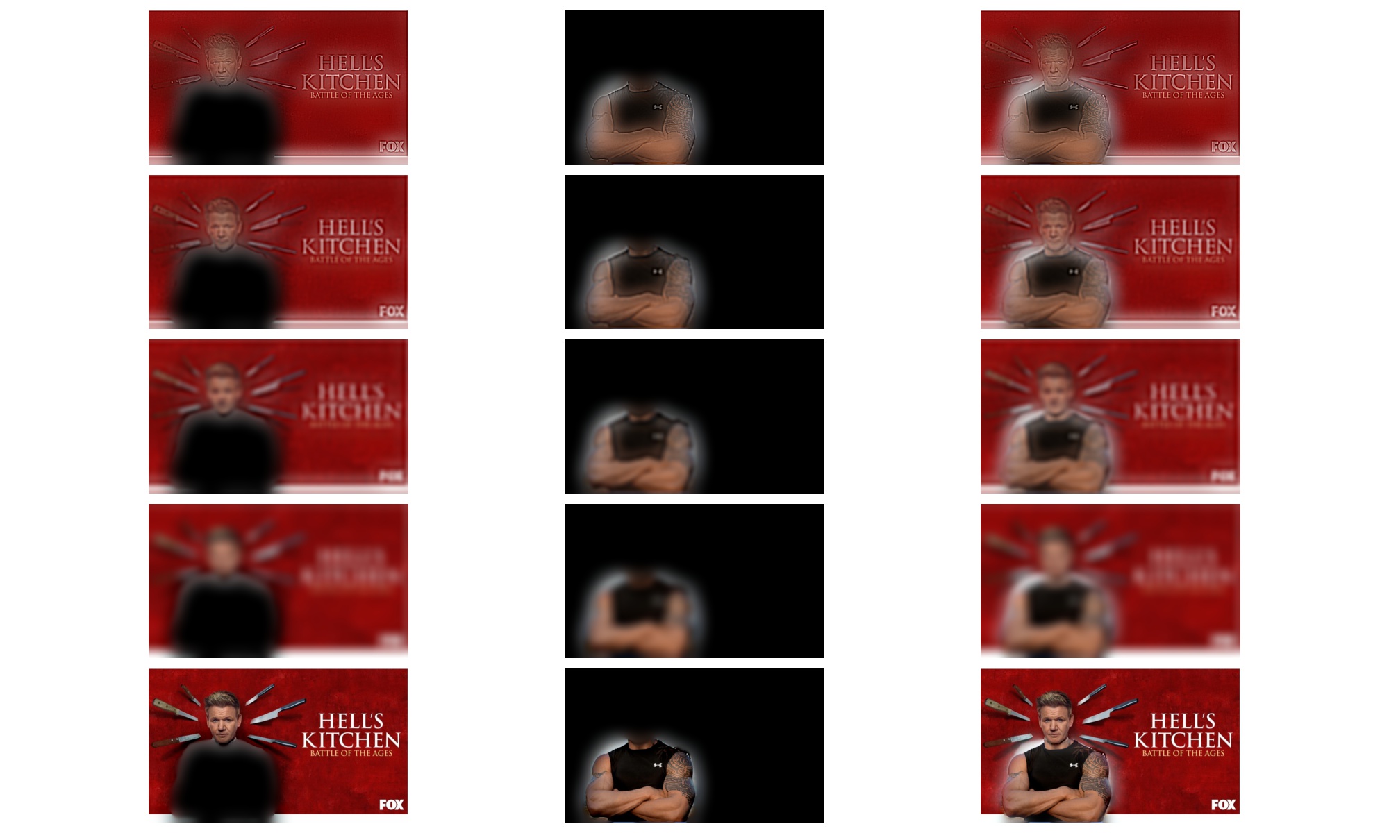
Hell Rock's Kitchen
What makes Hell's Kitchen even more intense? Gordon "The Rock" Ramsay!
 |  |  |
|---|
 |
|---|
Sadly, since their poses are not 100% the same, the white part on the right shoulder is hard to remove based on this method.